Gene Set Enrichment
→ Overview
Single differentially expressed genes on their own can be useful or informative - particularly if you have certain known markers or are looking for a potential therapeutic target. However, it is difficult to get the gestalt of the transcriptional landscape with single genes alone. Trying to stitch a pattern together ad-hoc is also quite challenging, given an individual gene can be involved in many processes, and there are so many processes to consider!
One way around this is to combine the changing patterns of many genes with some kind of database of known signatures. Stir some statistics in and you can measure the magnitude and statistical significance of this 'enrichment'.
There are many of these such analyses, but some of the ones I'm familiar with are gene ontology, pathway analysis, and gene set enrichment. Here we'll focus on Gene Set Enrichment Analysis (GSEA) and Gene Set Variation Analysis (GSVA), but the 'bones' of all these analyses are the same:
- Get some interesting genes (differentially expressed genes are a good start)
- Find a database that groups genes into meaningful categories (MSigDB, KEGG, gene ontology)
- Use some kind of statistical test to determine if your genes are more in a given category than you would expect by random chance
The specifics of step 3 are often handled for you by some kind of software package (thankfully, as this can be quite complex).
→ Gene Set Enrichment Analysis
I'm not going to cover differential expression - for that you can refer to the previous chapter. Instead, we'll start with already having differentially expressed genes in hand, particularly from the DESeq2::results stage.
This next section is just setup work. We're going to be looking at differentially expressed genes between bladder cancer cell lines that are known to be 'mesenchymal' (aggressive) and those that are known to be 'luminal papillary' (relatively indolent).
# If you have `pak`, you can install like so:
# pak::pak("McConkeyLab/cellebrate")
library(cellebrate)
library(DESeq2)
library(tidyverse)

cell_rna$clade <- factor(cell_rna$clade)

design(cell_rna) <- ~ clade

results <- cell_rna |>
  DESeq() |>
  results(c("clade", "Mesenchymal", "Luminal Papillary"))

results

# log2 fold change (MLE): clade Mesenchymal vs Luminal Papillary
# Wald test p-value: clade Mesenchymal vs Luminal.Papillary
# DataFrame with 18548 rows and 6 columns
#             baseMean log2FoldChange     lfcSE      stat      pvalue        padj
#            <numeric>      <numeric> <numeric> <numeric>   <numeric>   <numeric>
# TSPAN6   2440.115226      -1.504868  0.329809 -4.562843 5.04655e-06 8.78334e-05
# TNMD        0.505166       0.815607  2.270472  0.359223 7.19428e-01          NA
# DPM1     2181.151338       0.105421  0.280297  0.376104 7.06839e-01 8.35855e-01
# SCYL3     425.870650      -0.429055  0.191636 -2.238907 2.51620e-02 9.11602e-02
# C1orf112 1217.405323       0.313793  0.297827  1.053608 2.92063e-01 4.92163e-01
# ...              ...            ...       ...       ...         ...         ...
# MT-ND3       29804.2      -0.615508  0.289105  -2.12901  0.03325349   0.1115237
# MT-ND4      121143.9      -0.831135  0.296020  -2.80770  0.00498974   0.0265312
# MT-ND4L      19205.2      -0.730977  0.280703  -2.60409  0.00921174   0.0427057
# MT-ND5      113285.5      -0.662962  0.246290  -2.69179  0.00710689   0.0349475
# MT-ND6       31121.2      -0.696024  0.267147  -2.60540  0.00917672   0.0426275
I prefer working with a data.frame/tibble rather than a DataFrame (one of Bioconductor's objects), so I'll convert it. I'll also remove any genes that have NA log-fold-changes or p-values.
results_df <- results |>
  as_tibble(rownames = "gene") |>
  filter(!is.na(log2FoldChange), !is.na(padj))

results_df

# # A tibble: 16,430 × 7
#    gene     baseMean log2FoldChange lfcSE   stat      pvalue       padj
#    <chr>       <dbl>          <dbl> <dbl>  <dbl>       <dbl>      <dbl>
#  1 TSPAN6     2440.          -1.50  0.330 -4.56  0.00000505  0.0000878
#  2 DPM1       2181.           0.105 0.280  0.376 0.707       0.836
#  3 SCYL3       426.          -0.429 0.192 -2.24  0.0252      0.0912
#  4 C1orf112   1217.           0.314 0.298  1.05  0.292       0.492
#  5 FGR          17.3         -4.04  0.909 -4.44  0.00000895  0.000142
#  6 CFH        1386.          -4.08  0.972 -4.20  0.0000267   0.000362
#  7 FUCA2      3645.           1.29  0.505  2.55  0.0106      0.0476
#  8 GCLC       5655.          -2.35  0.452 -5.20  0.000000199 0.00000547
#  9 NFYA       1785.          -0.480 0.214 -2.24  0.0252      0.0912
# 10 STPG1       711.           1.03  0.330  3.12  0.00183     0.0121
# # ℹ 16,420 more rows
# # ℹ Use `print(n = ...)` to see more rows
Note that I'm not filtering for statistically significant genes, only genes that had valid test results. One of the touted advantages of gene set enrichment is the ability to find a strong signal from many weak (perhaps sub-statistically-significant) signals. However, I'm not entirely sure if the field is settled on this take - you're more than welcome to try it both ways (with all DEGS and with just significant DEGS).
→ GSEA
With step 1 (Get some interesting genes) done, we can move to step 2 - finding a database of gene groups. The work we need to do here is not finding the database (it's MSigDB), but getting a format suitable for downstream analysis.
MSigDB is a DataBase of Molecular Signatures. It has many collections - some of which are more manually assembled (so-called 'Hallmark' gene sets), and some of which are experimentally derived ('CGP' or 'chemical and genetic perturbations' is one). There's even Gene Ontology (GO). You can look at all the collections here.
I like to use the hallmark gene sets. It's a small collection (50 gene sets) and tends to span a wide enough gamut, and has enough eyes on it where I believe it's relatively well validated. However, with the approach I'm going to show you, switching between collections should be trivial.
The star of the show here is msigdbr, which will pull down genesets from MSigDB to your computer, locally. As such, the first time you run it it'll create a local database, which is a one time thing - it won't take long.
library(msigdbr)

hallmarks <- msigdbr(
  species = "Homo sapiens",
  collection = "H"
)

# Using `glimpse` (exported by `dplyr`) turns your data 'sideways'. While you don't get it in tabular format, it gives you a 'taste' of each column a bit easier.
glimpse(hallmarks)

# Rows: 8,209
# Columns: 15
# $ gs_cat             <chr> "H", "H", "H", "H", "H", "H", "…
# $ gs_subcat          <chr> "", "", "", "", "", "", "", "",…
# $ gs_name            <chr> "HALLMARK_ADIPOGENESIS", "HALLM…
# $ gene_symbol        <chr> "ABCA1", "ABCB8", "ACAA2", "ACA…
# $ entrez_gene        <int> 19, 11194, 10449, 33, 34, 35, 4…
# $ ensembl_gene       <chr> "ENSG00000165029", "ENSG0000019…
# $ human_gene_symbol  <chr> "ABCA1", "ABCB8", "ACAA2", "ACA…
# $ human_entrez_gene  <int> 19, 11194, 10449, 33, 34, 35, 4…
# $ human_ensembl_gene <chr> "ENSG00000165029", "ENSG0000019…
# $ gs_id              <chr> "M5905", "M5905", "M5905", "M59…
# $ gs_pmid            <chr> "26771021", "26771021", "267710…
# $ gs_geoid           <chr> "", "", "", "", "", "", "", "",…
# $ gs_exact_source    <chr> "", "", "", "", "", "", "", "",…
# $ gs_url             <chr> "", "", "", "", "", "", "", "",…
# $ gs_description     <chr> "Genes up-regulated during adip…
Note here that I've set the collection to H for Hallmarks, but it can take any top level collection name (H, C1, C2, C3, ..., C8). You can also specify a subcollection if you don't want all of C2, for instance, by specifying subcollection = "CGP". See ?msigdbr examples for a working example.
Further, it's important you set your species. If you don't, it will assume human and if your DEGs are not human, you will be sad when it doesn't match any of your supplied genes. Note that if your DEGs are not human, it will 'translate' the human gene to the nearest ortholog in the requested species. This is an important caveat, since the function of these genes and the pathways may not be conserved in your desired species.
Getting our genes into the format required for GSEA is trivial:
fgsea_pathways <- split(hallmarks$gene_symbol, hallmarks$gs_name)

# Showing you just the first six genes of the first 5 signatures. Each signature has a lot more than 5 genes.
lapply(fgsea_pathways, head)[1:5]

# $HALLMARK_ADIPOGENESIS
# [1] "ABCA1" "ABCB8" "ACAA2" "ACADL" "ACADM" "ACADS"

# $HALLMARK_ALLOGRAFT_REJECTION
# [1] "AARS1"  "ABCE1"  "ABI1"   "ACHE"   "ACVR2A" "AKT1"

# $HALLMARK_ANDROGEN_RESPONSE
# [1] "ABCC4"   "ABHD2"   "ACSL3"   "ACTN1"   "ADAMTS1" "ADRM1"

# $HALLMARK_ANGIOGENESIS
# [1] "APOH"   "APP"    "CCND2"  "COL3A1" "COL5A2" "CXCL6"

# $HALLMARK_APICAL_JUNCTION
# [1] "ACTA1" "ACTB"  "ACTC1" "ACTG1" "ACTG2" "ACTN1"
What's `split` doing?
You don't technically need to know what's going on in the split(...) business above, but it's a useful function and it's ultimately more satisfying to know what I'm doing rather than being led blindly by the nose.
split - as the name implies - splits a vector (here hallmarks$gene_symbol) into a list of vector 'fragments'. How it chooses to group the vector items into each fragment is determined by the second argument (here hallmarks$gs_name).
The result is a list of vectors of pathways, where each list item has the name of the grouping variable.
split is much more useful than just for this - I use it in combination with lapply to bust up a data.frame into groups and do SOMEthing to each group individually - essentially a poor-mans version of dplyr::group_by. See also tapply, which kind of does split and lapply all at once.
The last thing we need to do is prepare the differentially expressed genes for GSEA. This, too, is trivial. All we need is a named vector of log-fold-changes:
fgsea_input <- results_df$log2FoldChange
names(fgsea_input) <- results_df$gene

head(fgsea_input)

#     TSPAN6       DPM1      SCYL3   C1orf112        FGR        CFH
# -1.5048680  0.1054207 -0.4290554  0.3137928 -4.0384966 -4.0805457
Actually running GSEA is the easiest part:
library(fgsea)

fgsea_results <- fgsea(fgsea_pathways, fgsea_input)

glimpse(fgsea_results)
# Rows: 50
# Columns: 8
# $ pathway     <chr> "HALLMARK_ADIPOGENESIS", "HALLMARK_ALL…
# $ pval        <dbl> 9.870317e-01, 1.956522e-01, 3.014493e-…
# $ padj        <dbl> 1.000000e+00, 3.762542e-01, 5.197401e-…
# $ log2err     <dbl> 0.03099008, 0.11573445, 0.13427345, 0.…
# $ ES          <dbl> 0.2197217, 0.3536907, -0.3264371, 0.64…
# $ NES         <dbl> 0.7263282, 1.1511678, -1.0725414, 1.65…
# $ size        <int> 181, 153, 95, 32, 179, 40, 151, 104, 6…
# $ leadingEdge <list> <"ENPP2", "LPL", "MYLK", "PTGER3", "A…
fgsea gives us a row for each pathway we give it. The columns we're interested in tend to be pathway, padj (the p-value after adjustment for multiple-testing), and NES, the Normalized Enrichment Score. I plan to write a chapter detailing how GSEA works on a more technical level, but for now know that NES is the degree that the genes in this signature are present in either the most upregulated genes (positive NES) or the most downregulated genes (negative NES). It's 'normalized' because it accounts for the size of the gene set as well. The leadingEdge column can also be useful for determining which genes appear to be driving a given signature's enrichment, but we won't focus on it for this analysis.
I actually prefer to shake these results out into a tibble (just as with the DESeq2 results), but there are good reasons you may want to keep it in its current form, like the fgsea::plotGseaTable function (see here for more info). However, I'm just going to work with the table data to finish off the results for this section:
fgsea_results |>
  as_tibble() |>
  filter(padj < 0.05) |> # Only significant pathways
  arrange(desc(NES)) |> # Arrange by Normalized Enrichment Score
  select(-pval, -log2err, -leadingEdge) # To thin up the printed dataframe

# # A tibble: 11 × 5
#    pathway                                        padj     ES   NES  size
#    <chr>                                         <dbl>  <dbl> <dbl> <int>
#  1 HALLMARK_EPITHELIAL_MESENCHYMAL_TRANSITION 1.12e-18  0.723  2.40   188
#  2 HALLMARK_UV_RESPONSE_DN                    5.15e- 7  0.625  2.00   138
#  3 HALLMARK_ANGIOGENESIS                      3.03e- 2  0.649  1.63    32
#  4 HALLMARK_HYPOXIA                           5.68e- 3  0.472  1.56   185
#  5 HALLMARK_E2F_TARGETS                       5.76e- 3  0.463  1.54   192
#  6 HALLMARK_APICAL_JUNCTION                   8.74e- 3  0.467  1.54   179
#  7 HALLMARK_TNFA_SIGNALING_VIA_NFKB           3.03e- 2  0.439  1.46   190
#  8 HALLMARK_G2M_CHECKPOINT                    3.03e- 2  0.427  1.41   185
#  9 HALLMARK_ESTROGEN_RESPONSE_EARLY           3.03e- 2 -0.385 -1.39   185
# 10 HALLMARK_P53_PATHWAY                       2.10e- 2 -0.403 -1.45   186
# 11 HALLMARK_ESTROGEN_RESPONSE_LATE            5.68e- 3 -0.444 -1.60   186
From this, you can tell that the EMT signature is significantly upregulated in our mesenchymal cell lines versus the luminal papillary cell lines. This is consistent with our in-vitro observations - in general, luminal papillary lines fail to invade Matrigel and generally look more epithelial.
→ GSVA
GSEA uses differentially expressed genes, and thus requires you to group your data in some kind of comparison. Oftentimes this can make sense - if you did a drug/no drug experiment with some cell lines, for instance. Sometimes, however, you'd prefer not to arbitrarily set groups, or maybe you want to compare many groups at once.
GSVA allows you to do this by, ultimately, giving each sample a score for each signature, no differential expression required.
How's that work?
This is something else I'd like to write a chapter on. The fast and loose gist is:
For every GENE:
- Look at its expression across all samples to get a population distribution
- Convert that expression into (kind of) a z-score (using the distribution created above)
Now instead of expression, you have a bunch of z-score-ish things.
For every SAMPLE:
- Convert the 'z-scores' to ranks and arrange all the genes in descending order
Now you can treat these ranks kind of like you would log fold changes for GSEA, but now you have them for each sample instead of a result of a group comparison.
GSVA does not use differentially expressed genes. Instead, it uses expression values. While you can supply raw counts, I think you should probably normalize your counts first. This is easy with DESeq2:
normalized <- assay(vst(cell_rna))
I'm not going to print out normalized because it's a wall of text, but it's a 18548 row, 30 column matrix (where rows are genes, columns are samples) with each cell containing normalized expression value.
We can then feed this directly into gsvaParam, which in turn gets fed into gsva. Note that we can use the exact same format of pathways as an input as for fgsea, so we reuse fgsea_pathways.
library(GSVA)

params <- gsvaParam(normalized, fgsea_pathways)

results <- gsva(params)
Running this will result in a lot of warnings. Read the box below as to why.
HGNC symbols are for *you*, not the machines
This is a reminder to myself just as much as it is to inform you, but HGNC symbols - like ACTN1, GAPDH, or whatever - are more human-centric. They're recognizable, and sometimes imply (one) function of the gene product. However, they're imprecise and can even CHANGE over time. In general, stick with Entrez Gene IDs or Ensembl gene IDs. Sometimes you have to pick which one based on your downstream steps or upstream data, sometimes you get to choose.
Anyway, WHY this causes a headache with GSVA is because multiple Ensembl gene IDs map to single HGNC symbols (and sometimes the same Entrez IDs!):
# # A tibble: 2 × 3
#   gene_symbol ensembl_gene    human_entrez_gene
#   <chr>       <chr>                       <int>
# 1 MTCH2       ENSG00000109919             23788
# 2 MTCH2       ENSG00000285121             23788
Since our data only had gene symbols, we worked with the hand we were dealt and suffered the consequences. We could have removed the duplicates (and probably should have for any serious analysis) before doing GSEA and GSVA.
I'm also not printing out the results from this one and instead converting it directly into a tibble - I'm sparing you another wall of text:
results <- as_tibble(results, rownames = "pathway")

results[1:5] # Just the first 5 columns so it isn't so cramped

# A tibble: 50 × 5
#    pathway                            `1A6`  `253JP`  `5637`       BV
#    <chr>                              <dbl>    <dbl>   <dbl>    <dbl>
#  1 HALLMARK_ADIPOGENESIS            -0.220  -0.181   -0.188  -0.0899
#  2 HALLMARK_ALLOGRAFT_REJECTION      0.0373  0.102    0.315   0.0888
#  3 HALLMARK_ANDROGEN_RESPONSE       -0.142  -0.0942   0.0586 -0.158
#  4 HALLMARK_ANGIOGENESIS             0.246  -0.212    0.357  -0.0233
#  5 HALLMARK_APICAL_JUNCTION          0.237  -0.00814  0.159  -0.0669
#  6 HALLMARK_APICAL_SURFACE           0.270   0.0920   0.244  -0.0736
#  7 HALLMARK_APOPTOSIS               -0.0333 -0.165    0.188  -0.0889
#  8 HALLMARK_BILE_ACID_METABOLISM    -0.240   0.0145  -0.232  -0.00560
#  9 HALLMARK_CHOLESTEROL_HOMEOSTASIS -0.104  -0.222   -0.168  -0.289
# 10 HALLMARK_COAGULATION             -0.0245  0.0143   0.144   0.0263
# # ℹ 40 more rows
# # ℹ Use `print(n = ...)` to see more rows
As you can see, for every signature we put in, we get a row - and each sample gets its own value. These are super easy to work with - they're just numbers - so we have quite a bit of flexibility in how we present them.
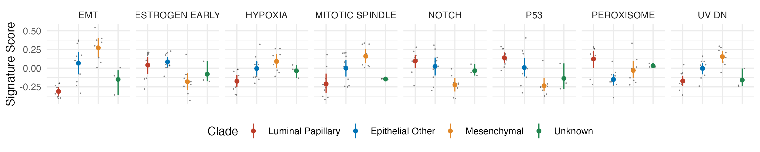
To cap this all off, I want to make a scatter plot showing EMT signature scores across the cell lines, colored by the subtypes we initially used for differential expression for GSEA. The details of how I do this are unimportant (I'm just showing a presentation example), but feel free to play around with it if you're curious.
library(broom) # For tidying statistical results
library(ggsci) # For pretty colors

results_long <- pivot_longer(results, -pathway, names_to = "cell")

# Adding back the columns that say which cell type is from which group (clade)
coldata_tibble <- as_tibble(colData(cell_rna))
results_with_calls <- left_join(results_long, coldata_tibble, by = "cell")

# Let's only plot the signatures for which the ANOVA p-value is < 0.01.

# Do an ANOVA on all of the signatures...
aov_results <- tapply(results_with_calls, ~pathway, \(x) tidy(aov(value ~ clade, x)))

# Loop through each pathway, see which is significant (the clade term), return TRUE or FALSE.
sig_pathways <- lapply(aov_results, \(x) x$p.value[1] < 0.01) |>
  unlist() |> # Turn it into a vector...
  which() |> # Kinda hacky, but returns only the values that are TRUE...
  names() # Get the names (pathways) of the TRUE items

sig_results <- results_with_calls |>
  filter(pathway %in% sig_pathways)

plotting_data <- sig_results |>
  # Clean up and abbreviate pathway names
  mutate(pathway = pathway |>
           str_remove_all("(HALLMARK_|_RESPONSE|_PATHWAY|_SIGNALING)") |>
           str_replace("EPITHELIAL_MESENCHYMAL_TRANSITION", "EMT") |>
           str_replace("_", " ")
         )

plot <- ggplot(plotting_data, aes(clade, value)) +
  facet_grid(~pathway) +
  geom_jitter(width = 0.2, size = 0.3, shape = 16, alpha = 0.5) +
  stat_summary(fun.data = "mean_cl_boot", size = 0.2, aes(color = clade)) +
  theme_minimal() +
  theme(
    axis.text.x = element_blank(),
    axis.title.x = element_blank(),
    legend.position = "bottom"
  ) +
  labs(y = "Signature Score", color = "Clade") +
  scale_color_nejm()

# ggsave("gsva-sig-pathways.png", plot, width = 25, height = 5, units = "cm")
→ Wrap Up
These are just a couple ways in which you can do gene set enrichment. Even within GSEA, you can do pathway and GO enrichment, or you can go for an entirely different database like KEGG. Proprietary software like Ingenuity Pathway Analysis can do this as well, but that's $$$. Personally, I think of this step as more exploratory than definitive: what you do with the implicated results - preferably with some kind of follow up experiment - is much more interesting.
This article doesn't go into much - if any - detail into the theory of GSEA or GSVA. I have aspirations to do separate articles explaining those, but give me a break!!! I'm tired all the time and apparently have a 'job'.
→ References
-
The
msigdbroverview. While writing this I was surprised to find thePathway enrichment analysissection, which I suppose would have been useful to know about previously. -
The
fgseavignette, which includes info like how to make enrichment plots and collapsing pathways, things I was not aware of before writing this! - The GSEA documentation, for interpreting GSEA statistics